Detection and high-frequency monitoring of methane emission point sources using Amazon SageMaker geospatial capabilities

Methane (CH4) is a major anthropogenic greenhouse gas that‘s a by-product of oil and gas extraction, coal mining, large-scale animal farming, and waste disposal, among other sources. The global warming potential of CH4 is 86 times that of CO2 and the Intergovernmental Panel on Climate Change (IPCC) estimates that methane is responsible for 30 percent of observed global warming to date . Rapidly reducing leakage of CH4 into the atmosphere represents a critical component in the fight against climate change. In 2021, the U.N. introduced The Global Methane Pledge at the Climate Change Conference (COP26), with a goal to take “fast action on methane to keep a 1.5C future within reach.” The Pledge has 150 signatories including the U.S. and EU.

Early detection and ongoing monitoring of methane sources is a key component of meaningful action on methane and is therefore becoming a concern for policy makers and organizations alike. Implementing affordable, effective methane detection solutions at scale – such as on-site methane detectors or aircraft-mounted spectrometers – is challenging, as they are often impractical or prohibitively expensive. Remote sensing using satellites, on the other hand, can provide the global-scale, high-frequency, and cost-effective detection functionality that stakeholders desire.

In this blog post, we show you how you can use Sentinel 2 satellite imagery hosted on the Amazon Web Services Registry of Open Data in combination with Amazon SageMaker geospatial capabilities to detect point sources of CH4 emissions and monitor them over time. Drawing on recent findings from the earth observation literature you will learn how you can implement a custom methane detection algorithm and use it to detect and monitor methane leakage from a variety of sites across the globe. This post includes accompanying code on GitHub that provides additional technical detail and helps you to get started with your own methane monitoring solution.

Traditionally, running complex geospatial analyses was a difficult, time-consuming, and resource-intensive undertaking. Amazon SageMaker geospatial capabilities make it easier for data scientists and machine learning engineers to build, train, and deploy models using geospatial data. Using SageMaker geospatial capabilities, you can efficiently transform or enrich large-scale geospatial datasets, accelerate model building with pre-trained machine learning (ML) models, and explore model predictions and geospatial data on an interactive map using 3D accelerated graphics and built-in visualization tools.

Remote sensing of methane point sources using multispectral satellite imagery

Satellite-based methane sensing approaches typically rely on the unique transmittance characteristics of CH4. In the visible spectrum, CH4 has transmittance values equal or close to 1, meaning it’s undetectable by the naked eye. Across certain wavelengths, however, methane does absorb light (transmittance <1), a property which can be exploited for detection purposes. For this, the short wavelength infrared (SWIR) spectrum (1500–2500 nm spectral range) is typically chosen, which is where CH4 is most detectable. Hyper- and multispectral satellite missions (that is, those with optical instruments that capture image data within multiple wavelength ranges (bands) across the electromagnetic spectrum) cover these SWIR ranges and therefore represent potential detection instruments. Figure 1 plots the transmittance characteristics of methane in the SWIR spectrum and the SWIR coverage of various candidate multispectral satellite instruments (adapted from this study).

Figure 1 – Transmittance characteristics of methane in the SWIR spectrum and coverage of Sentinel-2 multi-spectral missions

Many multispectral satellite missions are limited either by a low revisit frequency (for example, PRISMA Hyperspectral at approximately 16 days) or by low spatial resolution (for example, Sentinel 5 at 7.5 km x 7.5 km). The cost of accessing data is an additional challenge: some dedicated constellations operate as commercial missions, potentially making CH4 emission insights less readily available to researchers, decision makers, and other concerned parties due to financial constraints. ESA’s Sentinel-2 multispectral mission , which this solution is based on, strikes an appropriate balance between revisit rate (approximately 5 days), spatial resolution (approximately 20 m) and open access (hosted on the Amazon Web Services Registry of Open Data ).

Sentinel-2 has two bands that cover the SWIR spectrum (at a 20 m resolution): band-11 (1610 nm central wavelength) and band-12 (2190 nm central wavelength). Both bands are suitable for methane detection, while band-12 has significantly higher sensitivity to CH4 absorption (see Figure 1). Intuitively there are two possible approaches to using this SWIR reflectance data for methane detection. First, you could focus on just a single SWIR band (ideally the one that is most sensitive to CH4 absorption) and compute the pixel-by-pixel difference in reflectance across two different satellite passes. Alternatively, you use data from a single satellite pass for detection by using the two adjacent spectral SWIR bands that have similar surface and aerosol reflectance properties but have different methane absorption characteristics.

The detection method we implement in this blog post combines both approaches. We draw on recent findings from the earth observation literature and compute the fractional change in top-of-the-atmosphere (TOA) reflectance Δρ (that is, reflectance measured by Sentinel-2 including contributions from atmospheric aerosols and gases) between two satellite passes and the two SWIR bands; one baseline pass where no methane is present (base) and one monitoring pass where an active methane point source is suspected (monitor). Mathematically, this can be expressed as follows:

Equation (1)

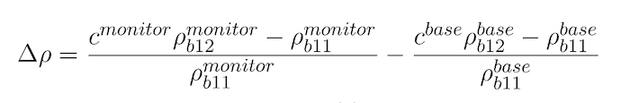
where ρ is the TOA reflectance as measured by Sentinel-2, c ^monitor and c ^base are computed by regressing TOA reflectance values of band-12 against those of band-11 across the entire scene (that is, ρ _b11 = c * ρ _b12 ). For more details, refer to this study on high-frequency monitoring of anomalous methane point sources with multispectral Sentinel-2 satellite observations .

Implement a methane detection algorithm with SageMaker geospatial capabilities

To implement the methane detection algorithm, we use the SageMaker geospatial notebook within Amazon SageMaker Studio. The geospatial notebook kernel is pre-equipped with essential geospatial libraries such as GDAL , GeoPandas , Shapely , xarray , and Rasterio , enabling direct visualization and processing of geospatial data within the Python notebook environment. See the getting started guide to learn how to start using SageMaker geospatial capabilities.

SageMaker provides a purpose-built API designed to facilitate the retrieval of satellite imagery through a consolidated interface using the SearchRasterDataCollection API call. SearchRasterDataCollection relies on the following input parameters:

• Arn : The Amazon resource name (ARN) of the queried raster data collection
• AreaOfInterest : A polygon object (in GeoJSON format) representing the region of interest for the search query
• TimeRangeFilter : Defines the time range of interest, denoted as {StartTime: <string>, EndTime: <string>}
• PropertyFilters : Supplementary property filters, such as specifications for maximum acceptable cloud cover, can also be incorporated

This method supports querying from various raster data sources which can be explored by calling ListRasterDataCollections . Our methane detection implementation uses Sentinel-2 satellite imagery , which can be globally referenced using the following ARN: arn:aws:sagemaker-geospatial:us-west-2:378778860802:raster-data-collection/public/nmqj48dcu3g7ayw8 .

This ARN represents Sentinel-2 imagery, which has been processed to Level 2A (surface reflectance, atmospherically corrected). For methane detection purposes, we will use top-of-atmosphere (TOA) reflectance data (Level 1C), which doesn’t include the surface level atmospheric corrections that would make changes in aerosol composition and density (that is, methane leaks) undetectable.

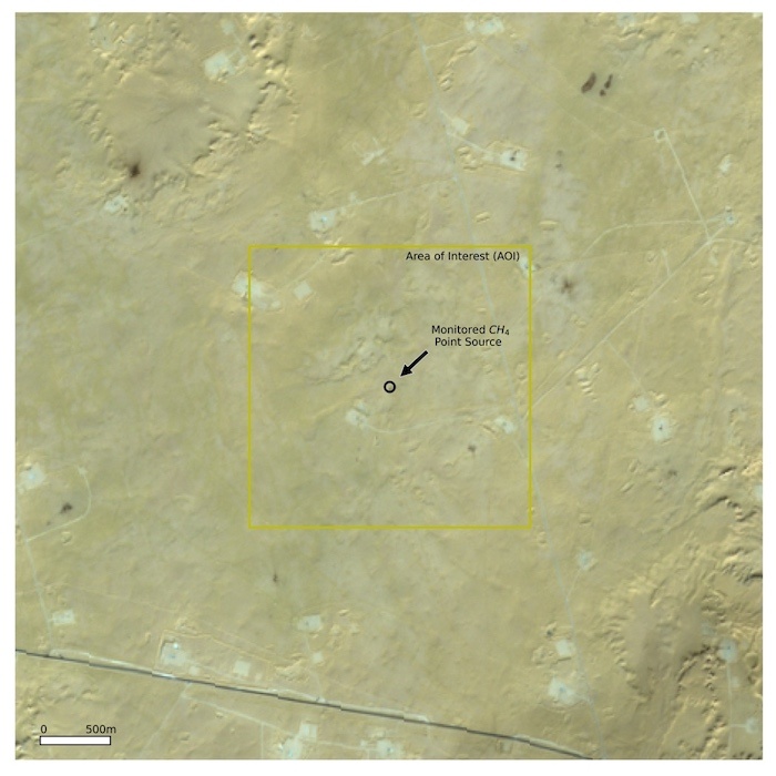
To identify potential emissions from a specific point source, we need two input parameters: the coordinates of the suspected point source and a designated timestamp for methane emission monitoring. Given that the SearchRasterDataCollection API uses polygons or multi-polygons to define an area of interest (AOI), our approach involves expanding the point coordinates into a bounding box first and then using that polygon to query for Sentinel-2 imagery using SearchRasterDateCollection .

In this example, we monitor a known methane leak originating from an oil field in Northern Africa. This is a standard validation case in the remote sensing literature and is referenced, for example, in this study. A fully executable code base is provided on the amazon-sagemaker-examples GitHub repository . Here, we highlight only selected code sections that represent the key building blocks for implementing a methane detection solution with SageMaker geospatial capabilities. See the repository for additional details.

We start by initializing the coordinates and target monitoring date for the example case.

#coordinates and date for North Africa oil field
#see here for reference: https://doi.org/10.5194/amt-14-2771-2021
point_longitude = 5.9053
point_latitude = 31.6585
target_date = '2019-11-20'
#size of bounding box in each direction around point
distance_offset_meters = 1500

The following code snippet generates a bounding box for the given point coordinates and then performs a search for the available Sentinel-2 imagery based on the bounding box and the specified monitoring date:

def bbox_around_point(lon, lat, distance_offset_meters):
    #Equatorial radius (km) taken from https://nssdc.gsfc.nasa.gov/planetary/factsheet/earthfact.html
    earth_radius_meters = 6378137
    lat_offset = math.degrees(distance_offset_meters / earth_radius_meters)
    lon_offset = math.degrees(distance_offset_meters / (earth_radius_meters * math.cos(math.radians(lat))))
    return geometry.Polygon([
        [lon - lon_offset, lat - lat_offset],
        [lon - lon_offset, lat + lat_offset],
        [lon + lon_offset, lat + lat_offset],
        [lon + lon_offset, lat - lat_offset],
        [lon - lon_offset, lat - lat_offset],
    ])

#generate bounding box and extract polygon coordinates
aoi_geometry = bbox_around_point(point_longitude, point_latitude, distance_offset_meters)
aoi_polygon_coordinates = geometry.mapping(aoi_geometry)['coordinates']

#set search parameters
search_params = {
    "Arn": "arn:aws:sagemaker-geospatial:us-west-2:378778860802:raster-data-collection/public/nmqj48dcu3g7ayw8", # Sentinel-2 L2 data
    "RasterDataCollectionQuery": {
        "AreaOfInterest": {
            "AreaOfInterestGeometry": {
                "PolygonGeometry": {
                    "Coordinates": aoi_polygon_coordinates
                }
            }
        },
        "TimeRangeFilter": {
            "StartTime": "{}T00:00:00Z".format(as_iso_date(target_date)),
            "EndTime": "{}T23:59:59Z".format(as_iso_date(target_date))
        }
    },
}
#query raster data using SageMaker geospatial capabilities
sentinel2_items = geospatial_client.search_raster_data_collection(**search_params)

The response contains a list of matching Sentinel-2 items and their corresponding metadata. These include Cloud-Optimized GeoTIFFs (COG) for all Sentinel-2 bands , as well as thumbnail images for a quick preview of the visual bands of the image. Naturally, it’s also possible to access the full-resolution satellite image (RGB plot), shown in Figure 2 that follows.

Figure 2 – Satellite image (RGB plot) of AOI

As previously detailed, our detection approach relies on fractional changes in top-of-the-atmosphere (TOA) SWIR reflectance. For this to work, the identification of a good baseline is crucial. Finding a good baseline can quickly become a tedious process that involves plenty of trial and error. However, good heuristics can go a long way in automating this search process. A search heuristic that has worked well for cases investigated in the past is as follows: for the past day_offset=n days, retrieve all satellite imagery, remove any clouds and clip the image to the AOI in scope. Then compute the average band-12 reflectance across the AOI. Return the Sentinel tile ID of the image with the highest average reflectance in band-12.

This logic is implemented in the following code excerpt. Its rationale relies on the fact that band-12 is highly sensitive to CH4 absorption (see Figure 1). A greater average reflectance value corresponds to a lower absorption from sources such as methane emissions and therefore provides a strong indication for an emission free baseline scene.

def approximate_best_reference_date(lon, lat, date_to_monitor, distance_offset=1500, cloud_mask=True, day_offset=30):
    
    #initialize AOI and other parameters
    aoi_geometry = bbox_around_point(lon, lat, distance_offset)
    BAND_12_SWIR22 = "B12"
    max_mean_swir = None
    ref_s2_tile_id = None
    ref_target_date = date_to_monitor   
        
    #loop over n=day_offset previous days
    for day_delta in range(-1 * day_offset, 0):
        date_time_obj = datetime.strptime(date_to_monitor, '%Y-%m-%d')
        target_date = (date_time_obj + timedelta(days=day_delta)).strftime('%Y-%m-%d')   
        
        #get Sentinel-2 tiles for current date
        s2_tiles_for_target_date = get_sentinel2_meta_data(target_date, aoi_geometry)
        
        #loop over available tiles for current date
        for s2_tile_meta in s2_tiles_for_target_date:
            s2_tile_id_to_test = s2_tile_meta['Id']
            #retrieve cloud-masked (optional) L1C band 12
            target_band_data = get_s2l1c_band_data_xarray(s2_tile_id_to_test, BAND_12_SWIR22, clip_geometry=aoi_geometry, cloud_mask=cloud_mask)
            #compute mean reflectance of SWIR band
            mean_swir = target_band_data.sum() / target_band_data.count()
            
            #ensure the visible/non-clouded area is adequately large
            visible_area_ratio = target_band_data.count() / (target_band_data.shape[1] * target_band_data.shape[2])
            if visible_area_ratio <= 0.7: #<-- ensure acceptable cloud cover
                continue
            
            #update maximum ref_s2_tile_id and ref_target_date if applicable
            if max_mean_swir is None or mean_swir > max_mean_swir: 
                max_mean_swir = mean_swir
                ref_s2_tile_id = s2_tile_id_to_test
                ref_target_date = target_date

    return (ref_s2_tile_id, ref_target_date)

Using this method allows us to approximate a suitable baseline date and corresponding Sentinel-2 tile ID. Sentinel-2 tile IDs carry information on the mission ID (Sentinel-2A/Sentinel-2B), the unique tile number (such as, 32SKA), and the date the image was taken among other information and uniquely identify an observation (that is, a scene). In our example, the approximation process suggests October 6, 2019 (Sentinel-2 tile: S2B_32SKA_20191006_0_L2A ), as the most suitable baseline candidate.

Next, we can compute the corrected fractional change in reflectance between the baseline date and the date we’d like to monitor. The correction factors c (see Equation 1 preceding) can be calculated with the following code:

def compute_correction_factor(tif_y, tif_x):
    
    #get flattened arrays for regression
    y = np.array(tif_y.values.flatten())
    x = np.array(tif_x.values.flatten())
    np.nan_to_num(y, copy=False)
    np.nan_to_num(x, copy=False)
        
    #fit linear model using least squares regression
    x = x[:,np.newaxis] #reshape
    c, _, _, _ = np.linalg.lstsq(x, y, rcond=None)

    return c[0]

The full implementation of Equation 1 is given in the following code snippet:

def compute_corrected_fractional_reflectance_change(l1_b11_base, l1_b12_base, l1_b11_monitor, l1_b12_monitor):
    
    #get correction factors
    c_monitor = compute_correction_factor(tif_y=l1_b11_monitor, tif_x=l1_b12_monitor)
    c_base = compute_correction_factor(tif_y=l1_b11_base, tif_x=l1_b12_base)
    
    #get corrected fractional reflectance change
    frac_change = ((c_monitor*l1_b12_monitor-l1_b11_monitor)/l1_b11_monitor)-((c_base*l1_b12_base-l1_b11_base)/l1_b11_base)
    return frac_change

Finally, we can wrap the above methods into an end-to-end routine that identifies the AOI for a given longitude and latitude, monitoring date and baseline tile, acquires the required satellite imagery, and performs the fractional reflectance change computation.

def run_full_fractional_reflectance_change_routine(lon, lat, date_monitor, baseline_s2_tile_id, distance_offset=1500, cloud_mask=True):
    
    #get bounding box
    aoi_geometry = bbox_around_point(lon, lat, distance_offset)
    
    #get S2 metadata
    s2_meta_monitor = get_sentinel2_meta_data(date_monitor, aoi_geometry)
    
    #get tile id
    grid_id = baseline_s2_tile_id.split("_")[1]
    s2_tile_id_monitor = list(filter(lambda x: f"_{grid_id}_" in x["Id"], s2_meta_monitor))[0]["Id"]
    
    #retrieve band 11 and 12 of the Sentinel L1C product for the given S2 tiles
    l1_swir16_b11_base = get_s2l1c_band_data_xarray(baseline_s2_tile_id, BAND_11_SWIR16, clip_geometry=aoi_geometry, cloud_mask=cloud_mask)
    l1_swir22_b12_base = get_s2l1c_band_data_xarray(baseline_s2_tile_id, BAND_12_SWIR22, clip_geometry=aoi_geometry, cloud_mask=cloud_mask)
    l1_swir16_b11_monitor = get_s2l1c_band_data_xarray(s2_tile_id_monitor, BAND_11_SWIR16, clip_geometry=aoi_geometry, cloud_mask=cloud_mask)
    l1_swir22_b12_monitor = get_s2l1c_band_data_xarray(s2_tile_id_monitor, BAND_12_SWIR22, clip_geometry=aoi_geometry, cloud_mask=cloud_mask)
    
    #compute corrected fractional reflectance change
    frac_change = compute_corrected_fractional_reflectance_change(
        l1_swir16_b11_base,
        l1_swir22_b12_base,
        l1_swir16_b11_monitor,
        l1_swir22_b12_monitor
    )
    
    return frac_change

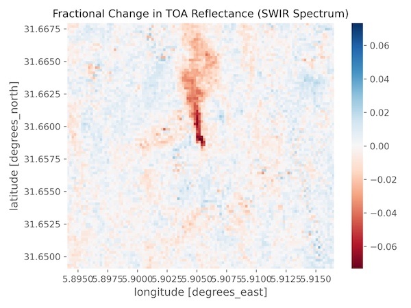
Running this method with the parameters we determined earlier yields the fractional change in SWIR TOA reflectance as an xarray.DataArray . We can perform a first visual inspection of the result by running a simple plot() invocation on this data array. Our method reveals the presence of a methane plume at the center of the AOI that was undetectable in the RGB plot seen previously.

Figure 3 – Fractional reflectance change in TOA reflectance (SWIR spectrum)

As a final step, we extract the identified methane plume and overlay it on a raw RGB satellite image to provide the important geographic context. This is achieved by thresholding, which can be implemented as shown in the following:

def get_plume_mask(change_in_reflectance_tif, threshold_value):
    cr_masked = change_in_reflectance_tif.copy()
    #set values above threshold to nan
    cr_masked[cr_masked > treshold_value] = np.nan 
    #apply mask on nan values
    plume_tif = np.ma.array(cr_masked, mask=cr_masked==np.nan) 
    
    return plume_tif

For our case, a threshold of -0.02 fractional change in reflectance yields good results but this can change from scene to scene and you will have to calibrate this for your specific use case. Figure 4 that follows illustrates how the plume overlay is generated by combining the raw satellite image of the AOI with the masked plume into a single composite image that shows the methane plume in its geographic context.

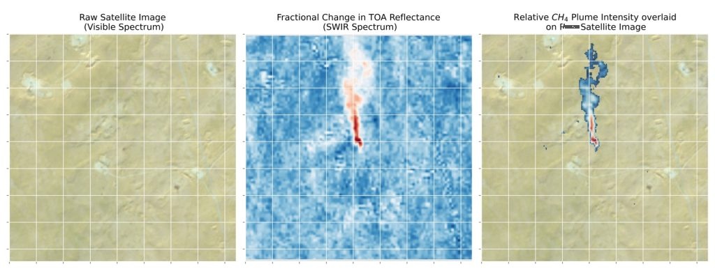
Figure 4 – RGB image, fractional reflectance change in TOA reflectance (SWIR spectrum), and methane plume overlay for AOI

Solution validation with real-world methane emission events

As a final step, we evaluate our method for its ability to correctly detect and pinpoint methane leakages from a range of sources and geographies. First, we use a controlled methane release experiment specifically designed for the validation of space-based point-source detection and quantification of onshore methane emissions . In this 2021 experiment, researchers performed several methane releases in Ehrenberg, Arizona over a 19-day period. Running our detection method for one of the Sentinel-2 passes during the time of that experiment produces the following result showing a methane plume:

Figure 5 – Methane plume intensities for Arizona Controlled Release Experiment

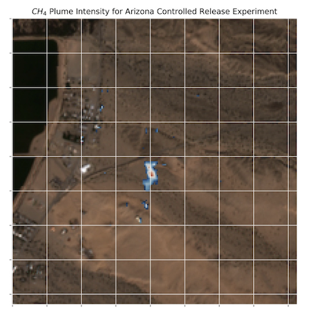
The plume generated during the controlled release is clearly identified by our detection method. The same is true for other known real-world leakages (in Figure 6 that follows) from sources such as a landfill in East Asia (left) or an oil and gas facility in North America (right).

Figure 6 – Methane plume intensities for an East Asian landfill (left) and an oil and gas field in North America (right)

In sum, our method can help identify methane emissions both from controlled releases and from various real-world point sources across the globe. This works best for on-shore point sources with limited surrounding vegetation. It does not work for off-shore scenes due to the high absorption (that is, low transmittance) of the SWIR spectrum by water . Given that the proposed detection algorithm relies on variations in methane intensity, our method also requires pre-leakage observations. This can make monitoring of leakages with constant emission rates challenging.

Clean up

To avoid incurring unwanted charges after a methane monitoring job has completed, ensure that you terminate the SageMaker instance and delete any unwanted local files.

Conclusion

By combining SageMaker geospatial capabilities with open geospatial data sources you can implement your own highly customized remote monitoring solutions at scale. This blog post focused on methane detection, a focal area for governments, NGOs and other organizations seeking to detect and ultimately avoid harmful methane emissions. You can get started today in your own journey into geospatial analytics by spinning up a Notebook with the SageMaker geospatial kernel and implement your own detection solution. See the GitHub repository to get started building your own satellite-based methane detection solution. Also check out the sagemaker-examples repository for further examples and tutorials on how to use SageMaker geospatial capabilities in other real-world remote sensing applications.

About the authors

Dr. Karsten Schroer is a Solutions Architect at Amazon Web Services. He supports customers in leveraging data and technology to drive sustainability of their IT infrastructure and build cloud-native data-driven solutions that enable sustainable operations in their respective verticals. Karsten joined Amazon Web Services following his PhD studies in applied machine learning & operations management. He is truly passionate about technology-enabled solutions to societal challenges and loves to dive deep into the methods and application architectures that underlie these solutions.

Janosch Woschitz is a Senior Solutions Architect at Amazon Web Services, specializing in geospatial AI/ML. With over 15 years of experience, he supports customers globally in leveraging AI and ML for innovative solutions that capitalize on geospatial data. His expertise spans machine learning, data engineering, and scalable distributed systems, augmented by a strong background in software engineering and industry expertise in complex domains such as autonomous driving.