
地理空间数据,包括许多气候和天气数据集,通常由政府和非营利组织以压缩文件格式发布,例如
网络通用数据表
(NetCDF) 或
Gridded
Binary (GRIB)。 这些格式中有许多是在云前世界中设计的,用户可以下载整个文件在本地计算机上进行分析。随着地理空间数据集复杂性和规模的持续增长,将文件放在一个地方,虚拟查询数据并仅下载本地所需的子集,这样既省时又更具成本效益。
与传统文件格式不同,云原生
Zarr
格式旨在虚拟高效地访问保存在中心位置的压缩数据块,例如来自亚马逊网络服务 (亚马逊云科技) 的
亚马逊简单存储服务
(Amazon S3)。
在本演练中,学习如何使用亚马逊 SageMa ker
笔记本
和
亚马逊云科技 Fargate 集群将 NetCDF 数据集转换为 Zar
r,并查询生成的 Zarr 存储,从而将时间序列查询所需的时间从几分钟缩短到几秒。
传统的地理空间数据格式
地理空间栅格数据文件将数据点与经纬度网格中的像元相关联。此类数据至少是二维的,但如果多个数据变量与每个像元相关联(例如,温度和风速),或者随着时间的推移记录变量或与海拔等附加维度相关联,则会增长到 N 维。
多年来,已经设计了许多文件格式来存储此类数据。1985 年创建的 GRIB 格式将数据存储为压缩二维记录的集合,每条记录对应一个时间步。但是,GRIB 文件不包含支持直接访问记录的元数据;检索单个变量的时间序列需要顺序访问每条记录。
NetCDF 于 1990 年推出,在 GRIB 的一些缺陷基础上进行了改进。NetCDF 文件包含支持更高效的数据索引和检索的元数据,包括远程打开文件和虚拟浏览其结构,而无需将所有内容加载到内存中。NetCDF 数据可以作为区块存储在文件中,从而实现对不同区块的并行读取和写入。自 2002 年起,NetCDF4 使用
分层数据格式版本 5 (HDF5
) 作为后端,提高了区块上并行 I/O 的速度。但是,由于单个文件中包含多个区块,NetCDF4 数据集的查询性能仍可能受到限制。
使用 Zarr 生成云原生地理空间数据
Zarr 文件格式将 N 维数据组织为组(数据集)和数组(数据集中的变量)的层次结构。每个数组的数据都存储为一组压缩的二进制块,每个区块都写入自己的文件。
将 Zarr 与 Amazon S3 搭配使用可实现毫秒级延迟的区块访问。区块读取和写入可以并行运行并根据需要进行扩展,既可以通过来自单台计算机的多线程或进程,也可以通过分布式计算资源(例如在
亚马逊弹性容器服务 (Amazon ECS) 中运行的容
器)进行扩展。将 Zarr 数据存储在 Amazon S3 中并应用分布式计算不仅可以避免数据下载时间和成本,而且通常是分析地理空间数据的唯一选择,因为这些数据太大而无法放入单台计算机的 RAM 或磁盘上。
最后,Zarr 格式包含可访问的元数据,允许用户远程打开和浏览数据集,并仅在本地下载所需的数据子集,例如分析的输出。下图显示了包含一个数组的 Zarr 组中包含的元数据文件和区块的示例。
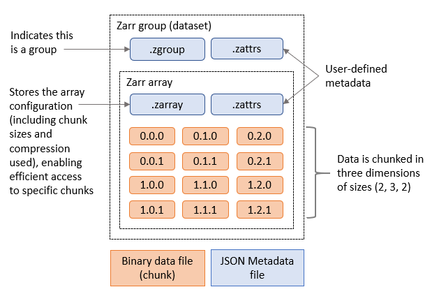
图 1。包含一个 Zarr 数组的 Zarr 组。
Zarr 与开源 P
angeo 技术堆栈
中的其他 Python 库紧密集成, 用于分析科学数据,例如 用于协调分布式并行计算作业的
Dask
和 用作处理标记 N 维
数组数据的接口的 xarray
。
Zarr 性能优势
亚马逊云科技 上的开放数据 注册表
包含许多广泛使用的地理空间数据集的 NetCDF 和 Zarr 版本,包括 ECMWF 再分析 v5 (ERA5) 数据集。
ERA5 包含自 2008 年以来在 31 千米纬度网格上多个高度的每小时气压、风速和气温数据。
我们比较了从ERA5的netCDF和Zarr版本中查询这三个变量在给定纬度和经度上一年、五、九和十三年的历史数据的平均时间。
|
Length of time series
|
Avg. NetCDF query time (seconds)
|
Avg. Zarr query time (seconds)
|
|
1 year
|
23.8
|
1.3
|
|
5 years
|
82.7
|
2.4
|
|
9 years
|
135.8
|
3.5
|
|
13 years
|
193.1
|
4.7
|
图 2。比较使用具有 10 个工作线程(8 个 vCPU、16 个 GM 内存)的 Dask 集群查询三个 ERA5 变量的平均时间。
请注意,这些测试并不是文件格式的真正一对一比较,因为每种格式使用的区块大小不同,结果也可能因网络条件而异。但是,它们与基准研究一致,
基准研究 表明
,与NetCDF相比,Zarr具有显著的性能优势。
尽管 亚马逊云科技 上的开放数据注册表包含许多流行的地理空间数据集的 Zarr 版本,但这些数据集的 Zarr 分块策略可能未针对组织的数据访问模式进行优化,或者组织可能拥有大量采用 NetCDF 格式的内部数据集。在这些情况下,他们可能希望从 NetCDF 文件转换为 Zarr。
搬到扎尔
将 NetCDF 文件转换为 Zarr 有几种选择:P
angeo-forge
配方、使用 Python
re
chunker 库和使用 xarray。
Pangeo-Forge 项目提供了预制
配方
,可以让你将一些 GRIB 或 NetCDF 数据集转换为 Zarr,而无需深入研究特定格式的底层细节。
为了更好地控制转换过程,你可以使用 rechunker 和 xarray 库。Rechunker 可以高效地操作保存在永久存储中的分块数组。由于 rechunker 使用中间文件存储器并且专为并行执行而设计,因此它可用于将大于工作内存的数据集从一种文件格式转换为另一种文件格式(例如从 NetCDF 转换为 Zarr),同时更改底层区块的大小。这使其成为将大型 NetCDF 数据集转换为优化的 Zarr 格式的理想之选。Xarray 可用于将较小的数据集转换为 Zarr 或将数据从 NetCDF 文件附加到现有 Zarr 存储,例如时间序列中的其他数据点(rechunker 目前不支持)。
最后,虽然从技术上讲不是 从 NetCDF
转换
到 Zarr 的选项,但 K
erchunk
python 库创建了索引文件,允许像访问 Zarr 存储一样访问 NetCDF 数据集,与单独使用 NetCDF 相比,无需创建新的 Zarr 数据集即可显著提高性能。
这篇博文的其余部分提供了使用 rechunker 和 xarray 将 NetCDF 数据集转换为 Zarr 的分步说明。
解决方案概述
该解决方案部署在 连接
互联网网关
的
亚马逊虚拟私有云
(Amazon VPC) 中。在私有子网内,它既部署了在
亚马逊云科技 Far gate
上运行的 Dask 集群,又部署了用于向 Dask 集群提交任务的
亚马逊 SageMaker 笔记本
实例。 在公有子网中,
NAT 网关
为来自 Dask 集群或笔记本实例的连接提供互联网接入(例如,在安装库时)。最后,
网络负载均衡器
(NLB) 允许访问 Dask 仪表板来监控 Dask 作业的进度。VPC 中的资源通过亚马逊 S3 VP
C 终端节点访问 亚马逊 S3
。
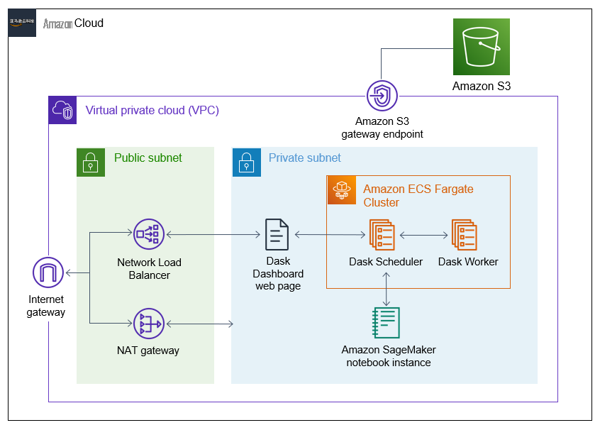
图 3。解决方案的架构图。
解决方案演练
以下是执行本演练所需步骤的简要概述,我们将对其进行更详细的介绍:
-
克隆
GitHub 存储库
。
-
使用
亚马逊云科技 云开发套件
(亚马逊云科技 CDK) 部署基础设施。
-
(可选)启用 Dask 控制面板。
-
在 SageMaker 笔记本实例上设置 Jupyter 笔记本。
-
使用 Jupyter 笔记本将 NetCDF 文件转换为 Zarr。
前四个步骤大部分是自动完成的,大约需要 45 分钟。设置完成后,运行 Jupyter 笔记本中的单元应该需要 30 分钟。
先决条件
在开始本演练之前,您应该具备以下先决条件:
-
一个
亚马逊云科技 账户
-
亚马逊云科技 身份和访问管理 (IAM) 有权执行本指南中的所有步骤
-
Python3
和 亚马逊云科技 CDK
安装
在您要部署解决方案的计算机上。
部署解决方案
第 1 步:克隆 GitHub 存储库
在终端中,运行以下代码来克隆 包含解决方案的
GitHub 存储库
。
git clone https://github.com/aws-samples/convert-netcdf-to-zarr.git
切换到存储库的根目录。
cd convert-netcdf-to-zarr
步骤 2:部署基础架构
从根目录运行以下代码来创建和激活虚拟环境并安装所需的库。(如果在 Windows 计算机上运行,则需要以 不同的方式
激活环境
。)
python3 -m venv .venv
source .venv/bin/activate
pip install -r requirements.txt
然后,运行以下代码来部署基础架构。
cdk deploy
此步骤首先构建将由 Dask 集群使用的 Docker 镜像。Docker 镜像完成后,CDK 会使用上述基础设施创建一个 ConvertToZarr CloudFormation 堆栈。当系统询问您是否要部署时,输入 “y”。此过程应持续 20—30 分钟。
步骤 3:(可选)启用 Dask 控制面板
Dask 仪表板为 Dask 分布式计算作业提供实时可视化和指标。仪表板不是 Jupyter 笔记本电脑正常工作所必需的,但有助于可视化作业和进行故障排除。Dask 仪表板在私有子网内的 Dask-Scheduler 任务端口上运行,因此我们使用 NLB 将来自互联网的请求转发到仪表板。
首先,复制 Dask 调度器的私有 IP 地址:
1。登录亚马逊 ECS 控制台。
2。选择
Dask-
Cluster。
3。选择 “
任务
” 选项卡。
4。选择具有
Dask-Schedul
er 任务定义的任务。
5。
在 “配置” 部分的 “
配置
” 选项卡中复制任务的
私有 IP 地址
。
现在,将 IP 地址添加为 NLB 的目标。
1。登录亚马逊 EC2 控制台。
2。在导航窗格中的
负载平衡
下 ,选择
目标组
。
3。选择以 C
onver-
dask 开头的目标组。
4。选择 “
注册目标
” 。
5。在步骤 1 中,确保选择了 “转换为 Zarr” VPC。在步骤 2 中,粘贴 Dask-Scheduler 的私有 IP 地址。该端口保持为 8787。在
下方选择 “ 包含为待处理
” 。
6。向下滚动到页面底部。选择
注册待处理目标
。几分钟后,目标的健康状态应从 “待处理” 更改为 “正常”,这表明您可以通过 Web 浏览器访问 Dask 控制面板。
最后,复制 NLB 的 DNS 名称。
1。登录亚马逊 EC2 控制台。
2。在导航窗格中的
负载平衡
下 ,选择
负载均衡器
。
3。
找到以
conve-daskd
开头的负载均衡器 并复制 DNS 名称。
4。将 DNS 名称粘贴到网络浏览器中以加载(空的)Dask 控制面板。
第 4 步:设置 Jupyter 笔记本
我们需要克隆 SageMaker 实例上的 GitHub 存储库,然后为 Jupyter 笔记本创建内核。
1。登录 SageMaker 控制台。
2。在导航窗格的 “
笔记本
” 下 ,选择 “
笔记本实例
” 。
3。
找到 “
转换为 Zarr 笔记本”,然后选择 “打开 Jupyt
er”。
4。
在 Jupyter 主页上,从右上角的 “
新建
” 菜单中选择 “终端”。
5。在终端中,运行以下命令。首先,切换到
SageMaker 目录:
cd SageMaker
接下来,克隆存储库:
git clone https://github.com/aws-samples/convert-netcdf-to-zarr.git
切换到存储库中的
笔记本
目录:
cd convert-netcdf-to-zarr/notebooks
6。最后,创建 Jupyter 内核作为新的 conda 环境。
conda env create --name zarr_py310_nb -f environment.yml
这应该需要 10-15 分钟。
步骤 5:将 netCDF 数据集转换为 Zarr
在 SageMaker 实例上,在 convert-netcdf 到 zarr/notebooks 文件夹中,打开 C
onvert-netCDF-to-Z
arr.ipynb。
这本 Jupyter 笔记本包含使用 rechunker 和 xarray 将每小时数据从
美国宇航局 MERRA-2
数据集(可从
亚马逊云科技 开放数据 注册表
获得 )从 NetCDF 转换为 Zarr 所需的所有步骤。让我们来看看一些关键的代码行。
下面的代码将笔记本注册为 Dask 集群的客户端。
DASK_SCHEDULER_URL = "Dask-Scheduler.local-dask:8786"
client = Client(DASK_SCHEDULER_URL)
然后,笔记本会生成一个包含两个月的每日 MERRA-2 NetCDF 文件 (nc_files_map) 的列表,并使用 Dask 集群打开这个带有数组的数据集。
ds_nc = xr.open_mfdataset(nc_files_map, engine='h5netcdf', chunks={}, parallel=True)
chunks 参数指示 xarray 将数据作为 Dask 数组存储在内存中,并且 parallel=True 告诉 Dask 在集群上并行打开 netCDF 文件。
该笔记本侧重于将数据集中一个变量 T2M(2 米处的气温)的数据从 netCDF 转换为 Zarr。T2M 的 x 数组输出显示,netCDF 区块大小为 (24、361、576)。
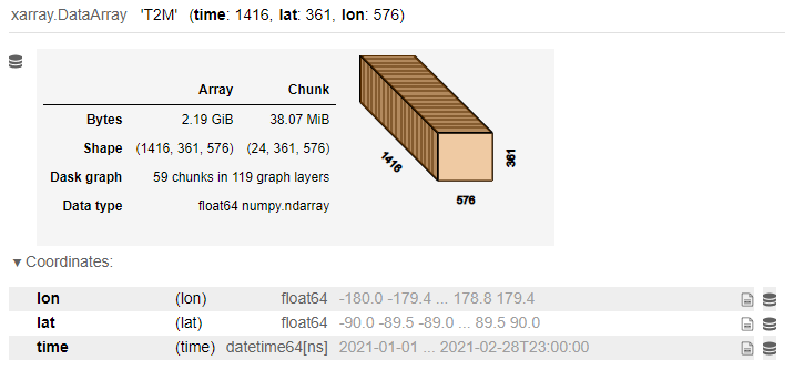
图 4。T2M 的 X 阵列输出。
查询 NetCDF 文件中两个月的给定纬度和经度的 T2M 数据需要 1-2 分钟。如果您启用了 Dask 控制面板,则可以在 Dask 集群上查看查询的进度。
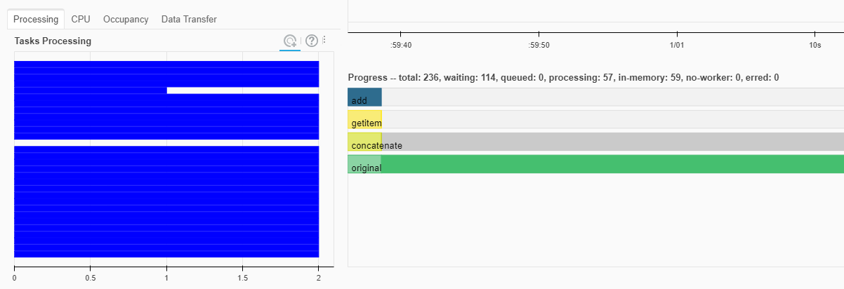
图 5。Dask 仪表板。
接下来,在开始 Zarr 转换之前,笔记本会为 Zarr 存储区创建一个包含新区块大小的字典(new_chunksizes_dict)。
# returns [“time”, “lat”, “lon”]
dims = ds_nc.dims.keys()

new_chunksizes = (1080, 90, 90)
new_chunksizes_dict = dict(zip(dims, new_chunksizes))
相对于NetCDF区块大小,新的Zarr区块大小(1080、90、90)在时间维度上更大,以减少在时间序列查询期间读取的区块数,而在其他两个维度上较小,以保持创建的区块的大小和数量保持在适当的级别。
下面的代码块显示了对 rechunk 函数的调用。传递给该函数的关键参数是要转换的 NetCDF 数据集 (ds_nc)、要转换的每个变量的目标区块大小(new_chunksizes_dict)(var_name,在本例中等于 T2M)、将要创建的 Zarr 存储的 S3 URI(zarr_store)。
ds_zarr = rechunk(
    ds_nc,
    target_chunks={
      var_name: new_chunksizes_dict,
      'time': None,'lat': None,'lon': None
    },
    max_mem='15GB',
    target_store = zarr_store,
    temp_store = zarr_temp
).execute()
Jupyter 笔记本包含对分块策略和传递给 rechunk 的参数的更详细的讨论。转换大约需要五分钟。
最后,笔记本代码显示了如何使用 xarray 向刚刚创建的 Zarr 存储区逐一添加一周的额外数据。这应该花费大约 10 分钟。生成的 Zarr 存储在 Amazon S3 上的文件结构如下所示。
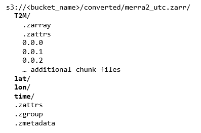
图 6。Zarr 将文件结构存储在亚马逊 S3 上。
结果?运行相同的查询来绘制两个月的指定纬度和经度的 T2M Zarr 数据所需的时间不到一秒,而使用 NetCDF 数据集大约需要 1-2 分钟。
正在清理
完成后,您可以通过从存储库的根目录运行以下代码来避免不必要的费用并删除使用该项目创建的 亚马逊云科技 资源:
cdk destroy
这将删除该项目创建的所有资源,S3 存储桶除外。要删除存储桶,请登录 亚马逊云科技 S3 控制台。选择存储桶并选择 “
清空
” 。存储桶清空后,再次选择该存储桶并选择
删除
。
结论
随着地理空间数据集规模的持续增长,将 Zarr 等云原生数据格式与 Amazon S3 等对象存储一起使用的性能优势也随之提高。尽管将数兆字节或更多的遗留数据转换为 Zarr 可能是一项艰巨的任务,但这篇文章提供了分步说明,以快速启动流程并解锁使用 Zarr 所带来的重大性能改进。
其他资源
有关在 亚马逊云科技 上处理基于阵列的地理空间数据的更多示例,请参阅:
-
使用亚马逊 SageMaker 和 亚马逊云科技 Fargate 在分布式 Dask 上进行机器学习
-
在 亚马逊云科技 上使用 Dask 和 Jupyter 分析太字节级的地理空间数据集
最后,采
用 Amaz on SageMaker 的地理空间机器
学习(现已提供预览版)允许客户高效地提取、转换和训练地理空间数据(包括卫星图像和位置数据)模型。它包括内置的基于地图的模型预测可视化效果,所有这些都可以在亚马逊 SageMaker Studio 笔记本电脑中使用。
订阅 亚马逊云科技 公共部门博客时事通讯
,
将来自公共部门的 亚马逊云科技 工具、解决方案和创新的最新信息发送到您的收件箱,或者
联系我们
。
请花几分钟时间在本次调查中分享您对 亚马逊云科技 公共部门博客的体验的见解
,我们将使用调查的反馈来创建更多符合读者偏好的内容。