这篇博客文章由Booking.com的莫兰·贝拉德夫、马诺斯·斯特吉亚迪斯和伊利亚·古塞夫共同撰写。
大型语言模型 (LLM) 凭借其理解和生成类人文本的能力,彻底改变了自然语言处理领域。LLM 接受过涵盖广泛主题和领域的广泛通用数据集的培训,他们利用其参数化知识在多个业务用例中执行越来越复杂和多功能的任务。此外,各公司越来越多地投入资源,通过少量学习和微调来定制LLM,以优化其在专业应用程序中的性能。
但是,LLM 令人印象深刻的性能是以大量的计算要求为代价的,这要归因于它们的大量参数和本质上是顺序的自回归解码过程。这种组合使得实现低延迟成为诸如实时文本完成、同声翻译或对话语音助手等用例的挑战,在这些用例中,亚秒级的响应时间至关重要。
研究人员开发了美杜莎,该框架通过增加额外的人才来同时预测多个代币,从而加快LLM推断。这篇文章演示了如何使用该框架的第一个版本Medusa-1通过在Amazon SageMaker AI上对其进行微调来加快LLM的速度,并确认了部署和简单负载测试的加速。Medusa-1 在不牺牲模型质量的情况下实现了大约两倍的推理加速,具体改进因模型大小和使用的数据而异。在这篇文章中,我们通过在样本数据集上观察到的1.8倍加速来演示其有效性。
美杜莎简介及其对 LLM 推理速度的好处
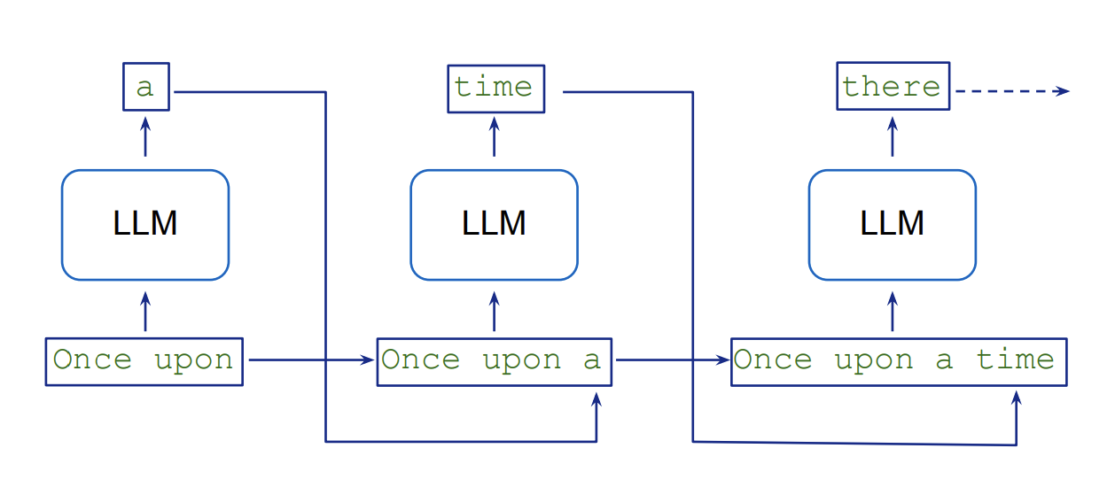
LLM 以顺序方式生成文本,这涉及自回归抽样,每个新代币都以先前的代币为条件。生成 K 个令牌需要连续执行 K 个模型。这种逐代币处理会带来固有的延迟和计算开销,因为模型需要为输出序列中的每个新令牌执行单独的向前传递。下图来自大型语言模型角色扮演游戏,说明了这一流程。
推测性解码通过使用更小、更快的草稿模型并行生成多个潜在的代币延续来应对这一挑战,然后由更大、更准确的目标模型进行验证。这种并行化加快了文本生成,同时保持了目标模型的质量,因为验证任务比自回归代币生成更快。有关该概念的详细解释,请参阅论文《使用推测采样加速大型语言模型解码》。推测性解码技术可以使用亚马逊SageMaker Jumpstart上的推理优化工具包来实现。
论文《美杜莎:具有多个解码头的简单 LLM 推理加速框架》介绍了美杜莎作为推测解码的替代方案。它没有添加单独的草稿模型,而是向 LLM 添加了额外的解码头,可以同时生成候选延续。然后使用基于树的注意力机制对这些候选人进行并行评估。这种并行处理减少了所需的顺序步骤的数量,从而缩短了推理时间。与推测性解码相比,美杜莎的主要优势在于,它无需获取和维护单独的草稿模型,同时实现更高的加速。例如,在MT-Bench数据集上进行测试时,该论文报告说,Medusa-2(美杜莎的第二个版本)将推理时间缩短了2.8倍。这比推测解码的性能要好,后者只能将同一数据集的推理时间缩短1.5倍。
美杜莎框架目前支持 Llama 和 Mistral 模型。尽管它提供了显著的速度改进,但它确实需要权衡内存(类似于推测解码)。例如,在 70 亿个参数的 Mistral 模型中添加五个美杜莎头会使总参数数增加 7.5 亿(每头 1.5 亿),这意味着这些额外的参数必须存储在 GPU 内存中,从而提高内存需求。但是,在大多数情况下,这种增加并不需要切换到更高的 GPU 内存实例。例如,您仍然可以使用具有 24 GB GPU 内存的ml.g5.4xlarge实例来托管 70 亿个参数的 Llama 或 Mistral 模型,以及额外的美杜莎头像。
培训美杜莎负责人需要额外的开发时间和计算资源,应将其纳入项目规划和资源分配。另一个需要提及的重要限制是,当前框架在部署在 Amazon SageMaker AI 终端节点上时,仅支持一个批量大小,这种配置通常用于低延迟应用程序。
下图来自美杜莎论文作者的FasterDecoding存储库,提供了美杜莎框架的可视化概述。
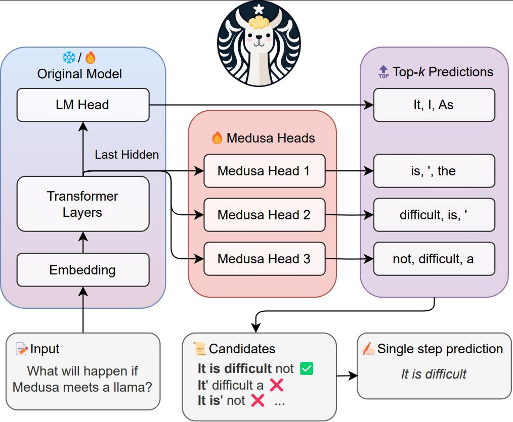
美杜莎有两个主要变体:
- Medusa-1 — 需要采用两阶段的方法,首先微调你的 LLM,然后添加美杜莎头像,在你的冷冻微调的 LLM 之上训练他们
- Medusa-2 — 稍后作为改进推出,可同时微调额外的磁头和主干 LLM 参数,从而有可能进一步提高延迟速度
美杜莎论文报告说,在不同大小的模型中,Medusa-1可以实现大约两倍的推理加速,Medusa-2的推理速度可以提高大约三倍。在Medusa-1中,预测与最初经过微调的LLM的预测相同。相比之下,在Medusa-2中,与简单微调LLM相比,我们观察到的结果可能略有不同,因为头部和骨干LLM参数是一起更新的。在这篇文章中,我们将重点介绍美杜莎-1。
解决方案概述
我们在解决方案中涵盖了以下步骤:
- 先决条件
- 加载和准备数据集
- 使用 SageMaker AI 训练作业微调 LLM
- 使用 SageMaker AI 训练任务,在经过微调的 LLM 上训练美杜莎的头部
- 在 SageMaker AI 终端上部署带有 Medusa 头部的经过微调的 LLM
- 演示 LLM 推理加速
通过遵循此解决方案,您可以加快应用程序中的 LLM 推断,从而缩短响应时间并改善用户体验。
先决条件
要自己构建解决方案,需要满足以下先决条件:
- 您需要一个具有 Amazon Identity and Access Management (IAM) 角色的亚马逊云科技账户,该角色有权管理作为解决方案一部分创建的资源(例如
AmazonSageMakerFullAccess和AmazonS3FullAccess)。有关详细信息,请参阅创建亚马逊云科技账户。
- 我们在亚马逊 SageMaker Studio 中使用 JupyterLab,该工作室在带有内核的实例上运行。
ml.t3.medium Python 3 (ipykernel)但是,您也可以使用亚马逊 SageMaker 笔记本实例(conda_pytorch_p310带内核)或您选择的任何集成开发环境 (IDE)。
- 请务必正确设置您的亚马逊云科技命令行接口 (亚马逊云科技CLI) 证书。有关更多信息,请参阅配置亚马逊云科技CLI。
- 该解决方案使用一个
ml.g5.4xlarge实例执行SageMaker AI训练任务,三个ml.g5.4xlarge实例用于SageMaker AI终端节点。如果需要,请申请增加配额,确保您的亚马逊云科技账户中有足够的容量来容纳此实例。另请查看按需实例的定价以了解相关成本。
- 要复制本文中演示的解决方案,你需要克隆这个 GitHub 存储库。在存储库中,你可以使用
medusa_1_train.ipynb笔记本来运行这篇文章中的所有步骤。该仓库是亚马逊 SageMaker 上原版《如何在 2024 年微调 LLM》的修改版。我们添加了简化的美杜莎训练代码,改编自最初的美杜莎存储库。
加载和准备数据集
现在您已经克隆了 GitHub 存储库并打开了medusa_1_train.ipynb笔记本,您将在笔记本中加载和准备数据集。我们鼓励你在笔记本中运行代码时阅读这篇文章。在这篇文章中,我们使用了一个名为 sql-create-create-context 的数据集,其中包含自然语言指令、架构定义和相应的 SQL 查询的示例。它包含 78,577 个自然语言查询、SQL CREATE TABLE 语句和使用 CREATE 语句作为上下文回答问题的 SQL 查询示例。出于演示目的,我们选择了 3,000 个样本并将其分成训练集、验证集和测试集。
您需要运行的 “加载并准备数据集” 部分medusa_1_train.ipynb来准备数据集以进行微调。我们还包括了一个数据探索脚本,用于分析输入和输出令牌的长度。在数据探索之后,我们会准备训练、验证和测试集,并将它们上传到亚马逊简单存储服务(Amazon S3)。
使用 SageMaker AI 训练作业微调 LLM
我们使用 Zephyr 7B β 模型作为我们的骨干 LLM。Zephyr是一系列经过培训的语言模型,可以充当有用的助手,而Zephyr 7B β是Mistral-7B-v0.1的微调版本,使用直接偏好优化在公开数据集和合成数据集上混合进行训练。
要启动 SageMaker AI 训练任务,我们需要使用 PyTorch 或 Hugging Face 估算器。在本例中,SageMaker AI 为我们启动和管理所有必要的亚马逊弹性计算云(亚马逊 EC2)实例,提供相应的容器,将数据从 S3 存储桶下载到容器并上传和运行指定的训练脚本。fine_tune_llm.py我们根据QLora论文选择超参数,但我们鼓励您尝试自己的组合。为了加快此代码的执行,我们将周期数设置为 1。但是,为了获得更好的结果,通常建议将周期数设置为至少 2 或 3。
from sagemaker.pytorch.estimator import PyTorch
from sagemaker.debugger import TensorBoardOutputConfig
import time
import os

def get_current_time():
    return time.strftime("%Y-%m-%d-%H-%M-%S", time.localtime())

def create_estimator(hyperparameters_dict, job_name, role, sess, train_scipt_path):
    metric=[
        {"Name": "loss", "Regex": r"'loss':\s*([0-9.]+)"},
        {"Name": "epoch", "Regex": r"'epoch':\s*([0-9.]+)"},
    ]

    tensorboard_s3_output_path = os.path.join(
       "s3://", sess.default_bucket(), job_name, 'tensorboard'
    )
    print("Tensorboard output path:", tensorboard_s3_output_path)

    tensorboard_output_config = TensorBoardOutputConfig(
        s3_output_path=tensorboard_s3_output_path,
        container_local_output_path=hyperparameters_dict['logging_dir']
    )
    estimator = PyTorch(
        sagemaker_session    = sess,
        entry_point          = train_scipt_path,    # train script
        source_dir           = 'train',      # directory which includes all the files needed for training
        instance_type        = 'ml.g5.4xlarge',   # instances type used for the training job, "local_gpu" for local mode
        metric_definitions   = metric,
        instance_count       = 1,                 # the number of instances used for training
        role                 = role,              # Iam role used in training job to access亚马逊云科技ressources, e.g. S3
        volume_size          = 300,               # the size of the EBS volume in GB
        framework_version      = '2.1.0',             # the pytorch_version version used in the training job
        py_version           = 'py310',           # the python version used in the training job
        hyperparameters      =  hyperparameters_dict,  # the hyperparameters passed to the training job
        disable_output_compression = True,        # not compress output to save training time and cost
        tensorboard_output_config = tensorboard_output_config
    )
    return estimator

# hyperparameters, which are passed into the training job
sft_hyperparameters = {
  ### SCRIPT PARAMETERS ###
  'train_dataset_path': '/opt/ml/input/data/train/train_dataset.json', # path where sagemaker will save training dataset
  'eval_dataset_path': '/opt/ml/input/data/eval/eval_dataset.json', # path where sagemaker will save evaluation dataset
  'model_id': model_id,
  'max_seq_len': 256,                               # max sequence length for model and packing of the dataset
  'use_qlora': True,                                 # use QLoRA model
  ### TRAINING PARAMETERS ###
  'num_train_epochs': 1,                             # number of training epochs
  'per_device_train_batch_size': 1,                  # batch size per device during training
  'gradient_accumulation_steps': 16,                  # number of steps before performing a backward/update pass
  'gradient_checkpointing': True,                    # use gradient checkpointing to save memory
  'optim': "adamw_8bit",                             # use fused adamw 8bit optimizer
  'logging_steps': 15,                               # log every 10 steps
  'save_strategy': "steps",                          # save checkpoint every epoch
  'save_steps': 15,
  'save_total_limit': 2,
  'eval_strategy': "steps",
  'eval_steps': 15,
  'learning_rate': 1e-4,                             # learning rate, based on QLoRA paper
  'bf16': True,                                      # use bfloat16 precision
  'max_grad_norm': 10,                              # max gradient norm based on QLoRA paper
  'warmup_ratio': 0.03,                              # warmup ratio based on QLoRA paper
  'lr_scheduler_type': "constant",                   # use constant learning rate scheduler
  'output_dir': '/opt/ml/checkpoints/',              # Temporary output directory for model checkpoints
  'merge_adapters': True,                            # merge LoRA adapters into model for easier deployment
  'report_to': "tensorboard",                        # report metrics to tensorboard
  'logging_dir': "/opt/ml/output/tensorboard"        # tensorboard logging directory
}

sft_job_name = f"sft-qlora-text-to-sql-{get_current_time()}"
data = {
    'train': train_dataset_path,
    'eval': eval_dataset_path
}

sft_estimator = create_estimator(sft_hyperparameters, sft_job_name, role, sess, "fine_tune_llm.py")

sft_estimator.fit(job_name=sft_job_name, inputs=data, wait=False)
当我们的训练任务在大约 1 小时后成功完成后,我们可以使用经过微调的模型工件进行下一步,在上面训练美杜莎的头部。要在 Tensorboard 中实现训练指标的可视化,您可以按照本文档中的指导进行操作:使用 TensorBoard 应用程序加载和可视化输出张量
使用 SageMaker AI 训练作业,在《冰雪奇缘》微调的 LLM 之上训练美杜莎的头部
为了训练美杜莎头像,我们可以重复使用前面提到的功能来启动训练任务。我们根据美杜莎论文报道的内容和经过几次实验后发现表现优秀的参数相结合来选择超参数。我们将美杜莎头的数量设置为 5,并按照论文的建议使用了 8 位 AdamW 优化器。为简单起见,我们使用恒定调度器保持了 1e-4 的恒定学习率,与之前的微调步骤类似。尽管本文建议提高学习率和使用余弦调度器,但我们发现我们选择的超参数组合在该数据集上表现良好。但是,我们鼓励您尝试自己的超参数设置,以获得更好的结果。
# hyperparameters, which are passed into the training job
medusa_hyperparameters = {
  ### SCRIPT PARAMETERS ###
  'train_dataset_path': '/opt/ml/input/data/train/train_dataset.json', # path where sagemaker will save training dataset
  'eval_dataset_path': '/opt/ml/input/data/eval/eval_dataset.json', # path where sagemaker will save evaluation dataset
  'model_path': '/opt/ml/input/data/fine-tuned-model/',
  'max_seq_len': 256,                               # max sequence length for model and packing of the dataset
  'medusa_num_heads': 5,
  ### TRAINING PARAMETERS ###
  'num_train_epochs': 3,                             # number of training epochs
  'per_device_train_batch_size': 1,                  # batch size per device during training
  'gradient_accumulation_steps': 16,                  # number of steps before performing a backward/update pass
  'gradient_checkpointing': True,                    # use gradient checkpointing to save memory
  'optim': "adamw_8bit",                             # use fused adamw 8bit optimizer
  'logging_steps': 15,                               # log every 10 steps
  'save_strategy': "steps",                          # save checkpoint every epoch
  'save_steps': 15,
  'save_total_limit':2,
  'eval_strategy': "steps",
  'eval_steps': 15,
  'learning_rate': 1e-4,                             # learning rate
  'bf16': True,                                      # use bfloat16 precision
  'max_grad_norm': 10,                              # max gradient norm based on QLoRA paper
  'warmup_ratio': 0.03,                              # warmup ratio based on QLoRA paper
  'lr_scheduler_type': "constant",                   # use constant learning rate scheduler
  'output_dir': '/opt/ml/checkpoints/',              # Temporary output directory for model checkpoints
  'report_to': "tensorboard",                        # report metrics to tensorboard
  'logging_dir': "/opt/ml/output/tensorboard"        # tensorboard logging directory
}

medusa_train_job_name = f"medusa-text-to-sql-{get_current_time()}"
data = {
    'train': train_dataset_path,
    'eval': eval_dataset_path,
    'fine-tuned-model': fine_tuned_model_path
}

medusa_estimator = create_estimator(medusa_hyperparameters, medusa_train_job_name, role, sess, "train_medusa_heads.py")

medusa_estimator.fit(job_name=medusa_train_job_name, inputs=data, wait=False)
我们发现,在3个周期之后,美杜莎头部的评估损失正在趋于一致,这可以在下图的TensorBoard图表中观察到。

除了超参数之外,主要区别在于我们train_medusa_heads.py作为训练切入点传递,我们首先添加美杜莎头像,然后冻结经过微调的 LLM,然后创建自定义 MedusaSftTrainer 类,这是变形金刚 SFTTrainer 的子类。
# Add medusa heads and freeze base model
add_medusa_heads(
    model,
    medusa_num_heads=script_args.medusa_num_heads,
)
freeze_layers(model)
model.config.torch_dtype = torch_dtype
model.config.use_cache = False

logger.info("Finished loading model and medusa heads")

tokenizer = AutoTokenizer.from_pretrained(script_args.model_path, use_fast=True)
tokenizer.pad_token = tokenizer.eos_token

################
# Training
################
trainer = MedusaSFTTrainer(
    model=model,
    args=training_args,
    train_dataset=train_dataset,
    eval_dataset=eval_dataset,
    max_seq_length=script_args.max_seq_length,
    tokenizer=tokenizer,
    dataset_kwargs={
        "add_special_tokens": False,  # We template with special tokens
        "append_concat_token": False,  # No need to add additional separator token
    },
    medusa_num_heads=script_args.medusa_num_heads,
    medusa_heads_coefficient=script_args.medusa_heads_coefficient,
    medusa_decay_coefficient=script_args.medusa_decay_coefficient,
    medusa_scheduler=script_args.medusa_scheduler,
    train_only_medusa_heads=script_args.train_only_medusa_heads,
    medusa_lr_multiplier=script_args.medusa_lr_multiplier
)
trainer.train()
在add_medusa_heads()函数中,我们添加了美杜莎头部的残留方块,同时重写了模型的前向传递,以确保不训练冰冻骨干 LLM:
def add_medusa_heads(
    model,
    medusa_num_heads,
):
    """
    Args:
        model (nn.Module): The base language model to be used.
        medusa_num_heads (int, optional): Number of additional tokens to predict
    """
    hidden_size = model.lm_head.weight.shape[-1]
    vocab_size = model.lm_head.weight.shape[0]
    model.config.medusa_num_layers = 1
    model.config.medusa_num_heads = medusa_num_heads
    model.medusa_num_heads = medusa_num_heads
    # Create a list of Medusa heads
    model.medusa_heads = nn.ModuleList(
        [
            nn.Sequential(
                ResBlock(hidden_size),
                nn.Linear(hidden_size, vocab_size, bias=False),
            )
            for _ in range(medusa_num_heads)
        ]
    )

    # Ensure medusa_head's dtype and device align with the base_model
    model.medusa_heads.to(model.dtype).to(model.device)
    logger.info(f"Loading medusa heads in {str(model.dtype)} to device {model.device}")

    for i in range(medusa_num_heads):
        # Initialize the weights of each medusa_head using the base model's weights
        model.medusa_heads[i][-1].weight.data[:] = model.lm_head.weight.data[:]

    def forward(
        self,
        input_ids: torch.LongTensor = None,
        attention_mask: Optional[torch.Tensor] = None,
        position_ids: Optional[torch.LongTensor] = None,
        past_key_values: Optional[List[torch.FloatTensor]] = None,
        inputs_embeds: Optional[torch.FloatTensor] = None,
        labels: Optional[torch.LongTensor] = None,
        use_cache: Optional[bool] = None,
        output_attentions: Optional[bool] = None,
        output_hidden_states: Optional[bool] = None,
        return_dict: Optional[bool] = None,
        train_only_medusa_heads: bool = False,
    ):
        """Forward pass of the MedusaModel.
        Returns:
            torch.Tensor: A tensor containing predictions from all Medusa heads.
            (Optional) Original predictions from the base model's LM head.
        """
        maybe_grad = torch.no_grad() if train_only_medusa_heads else nullcontext()
        with maybe_grad:
            outputs = self.model(
                input_ids=input_ids,
                attention_mask=attention_mask,
                position_ids=position_ids,
                past_key_values=past_key_values,
                inputs_embeds=inputs_embeds,
                use_cache=use_cache,
                output_attentions=output_attentions,
                output_hidden_states=output_hidden_states,
                return_dict=return_dict,
            )
            hidden_states = outputs[0]
            medusa_logits = [self.lm_head(hidden_states)]
        for i in range(self.medusa_num_heads):
            medusa_logits.append(self.medusa_heads[i](hidden_states))
        return torch.stack(medusa_logits, dim=0)

    model.forward = types.MethodType(forward, model)
模型训练完成(需要 1 小时)后,我们会准备模型工件以供部署并上传到 Amazon S3。您的最终模型工件包含base-model前缀下方经过微调的原始模型,以及名为的文件中经过训练的美杜莎头像。medusa_heads.safetensors
在 SageMaker AI 终端上部署带有 Medusa 头部的经过微调的 LLM
文本生成推断 (TGI) 服务器支持美杜莎框架。在用美杜莎头部训练了LLM之后,我们使用TGI设置的Hugging Face推理容器将其部署到SageMaker AI实时终端节点。
首先,我们创建一个 SageMaker AI HuggingFaceModel 对象,然后使用以下函数将模型部署到端点:
import json
from sagemaker.huggingface import HuggingFaceModel, get_huggingface_llm_image_uri


def deploy_model(endpoint_name, instance_type, model_s3_path=None, hf_model_id=None):
    llm_image = get_huggingface_llm_image_uri(
      "huggingface",
      version="2.2.0",
      session=sess,
    )

    print(f"llm image uri: {llm_image}")

    model_data = None
    if model_s3_path:
        model_data = {'S3DataSource': {'S3Uri': model_s3_path, 'S3DataType': 'S3Prefix', 'CompressionType': 'None'}}
        hf_model_id = "/opt/ml/model"
    else:
        assert hf_model_id, "You need to provide either pretrained HF model id, or S3 model data to deploy"
    config = {
      'HF_MODEL_ID': hf_model_id,  # path to where sagemaker stores the model
      'SM_NUM_GPUS': json.dumps(1),  # Number of GPU used per replica
      'MAX_INPUT_LENGTH': json.dumps(1024),  # Max length of input text
      'MAX_TOTAL_TOKENS': json.dumps(2048),  # Max length of the generation (including input text)
    }

    llm_model = HuggingFaceModel(
      name=endpoint_name,
      role=role,
      image_uri=llm_image,
      model_data=model_data,
      env=config
    )

    deployed_llm = llm_model.deploy(
      endpoint_name=endpoint_name,
      initial_instance_count=1,
      instance_type=instance_type,
      container_startup_health_check_timeout=300,
    )
    return deployed_llm
我们在三个 SageMaker AI 端点上部署了三个 LLM:
- 未经微调的基础 LLM
- 我们微调的 LLM
- 经过微调的 LLM 还训练了美杜莎的负责人
您可以使用我们在笔记本中包含的函数并行部署这三个模型,也可以通过运行以下代码逐一部署模型:
base_deployed_llm = deploy_model( f"base-{get_current_time()}", instance_type="ml.g5.4xlarge", model_s3_path=None, hf_model_id=model_id )
sft_deployed_llm = deploy_model( f"sft-{get_current_time()}", instance_type="ml.g5.4xlarge", model_s3_path=fine_tuned_model_path )
medusa_deployed_llm = deploy_model( f"medusa-{get_current_time()}", instance_type="ml.g5.4xlarge", model_s3_path=medusa_trained_model_path )
在每个端点的状态变为InService(大约需要 15 分钟)后,我们可以调用它们进行推断。我们发送以下输入:
“You are a text to SQL query translator. Users will ask you questions in English and you will generate a SQL query based on the provided SCHEMA. SCHEMA: CREATE TABLE table_name_32 (time VARCHAR, heat VARCHAR, name VARCHAR)
What was Liu Limin's time in heat 4?“
我们可以观察到以下回应:
- 基本的 LLM 响应包含不需要的额外单词:
“To retrieve the time of Liu Limin in heat 4 based on the provided SCHEMA, we need to write a SQL query. Since the table name is not provided, let 's assume it's "my_table". Assuming the table has a primary key (which is not mentioned in the SCHEMA), we can join the table with itself to compare the heat and name of Liu Limin in heat 4 with all the records in the table. Here's the SQL query: ``sql SELECT t1.time FROM my_table t1 JOIN my_table t2 ON t1.name = t2.name AND t2.heat = 4 WHERE t1.name = 'Liu Limin' AND t1.heat <> 4; ` Explanation: 1. We're selecting the time` column from the first table (t1) in the FROM clause. 2. We're joining the table with itself (my_table t1 JOIN my_table t2) to compare the name and heat of Liu Limin in heat 4 with all the records in the table. 3. We're filtering the results using the WHERE clause. We're selecting only the records where the name is 'Liu Limin' and the heat is not equal to 4 (i.e., not heat 4). This is to ensure that we're selecting the time of Liu Limin in heat 3. Note: This query assumes that the table has a unique primary key. If the table doesn't have a primary key, you may need to add additional conditions to the JOIN and WHERE clauses to ensure that we're selecting the correct records.“
- 经过微调的 LLM 响应得到了显著改善,并且仅包含所需的输出:
'SELECT time FROM table_name_32 WHERE heat = 4 AND name = "liu limin"'
- 由训练有素的美杜莎头部进行微调的 LLM 提供的响应与微调模型完全相同,这表明 Medusa-1 在设计上保持了原始模型的输出(质量):
'SELECT time FROM table_name_32 WHERE heat = 4 AND name = "liu limin"'
演示 LLM 推理加速
为了衡量推理速度的改进,我们使用以下代码比较了部署的微调LLM和带有美杜莎头部的微调LLM的响应时间,在450次测试观测结果中:
import time
import numpy as np
from tqdm import tqdm

def request(sample, deployed_llm):
    prompt = tokenizer.apply_chat_template(sample, tokenize=False, add_generation_prompt=True)
    outputs = deployed_llm.predict({
      "inputs": prompt,
      "parameters": {
        "max_new_tokens": 512,
        "do_sample": False,
        "return_full_text": False,
      }
    })
    return {"role": "assistant", "content": outputs[0]["generated_text"].strip()}

def predict(deployed_llm, test_dataset):
    predicted_answers = []
    latencies = []

    for sample in tqdm(test_dataset):
        start_time = time.time()
        predicted_answer = request(sample["messages"][:2], deployed_llm)
        end_time = time.time()

        latency = end_time - start_time
        latencies.append(latency)
        predicted_answers.append(predicted_answer)

    # Calculate p90 and average latencies
    p90_latency = np.percentile(latencies, 90)
    avg_latency = np.mean(latencies)

    print(f"P90 Latency: {p90_latency:.2f} seconds")
    print(f"Average Latency: {avg_latency:.2f} seconds")

    return predicted_answers
首先,我们使用经过微调的 LLM 进行预测:
sft_predictions = predict(sft_deployed_llm, test_dataset)
P90 Latency: 1.28 seconds
Average Latency: 0.95 seconds
然后,我们使用带有美杜莎头像的微调LLM进行预测:
medusa_predictions = predict(medusa_deployed_llm, test_dataset)
P90 Latency: 0.80 seconds
Average Latency: 0.53 seconds
预测运行应分别花费大约 8 分钟和 4 分钟。我们可以观察到,平均延迟从 950 毫秒减少到 530 毫秒,提高了 1.8 倍。如果您的数据集包含更长的输入和输出,则可以实现更高的改进。在我们的数据集中,我们平均只有18个输入令牌和30个输出令牌。
我们想再次强调,使用这种技术,输出质量可以完全保持,所有的预测输出都是一样的。对于有美杜莎头像和没有美杜莎头像的测试集,450个观测结果的模型响应是相同的:
match_percentage = sum(a["content"] == b["content"] for a, b in zip(sft_predictions, medusa_predictions)) / len(sft_predictions) * 100
print(f"Predictions with the fine-tuned model with medusa heads are the same as without medusa heads: {match_percentage:.2f}% of test set ")

Predictions with fine-tuned model with medusa heads are the same as without medusa heads: 100.00% of test set
在运行中,你可能会注意到一些观测值不完全匹配,并且由于在 GPU 上进行优化导致浮点运算出现小错误,你可能会得到 99% 的匹配率。
清理
在本实验结束时,别忘了删除你创建的 SageMaker AI 端点:
base_deployed_llm.delete_model()
base_deployed_llm.delete_endpoint()
sft_deployed_llm.delete_model()
sft_deployed_llm.delete_endpoint()
medusa_deployed_llm.delete_model()
medusa_deployed_llm.delete_endpoint()
结论
在这篇文章中,我们演示了如何在亚马逊 SageMaker AI 上使用 Medusa-1 技术微调和部署带有美杜莎头像的 LLM,以加速 LLM 推断。通过使用该框架和 SageMaker AI 可扩展基础架构,我们展示了如何在保持模型质量的同时实现 LLM 推理的两倍加速。该解决方案特别适用于需要低延迟文本生成的应用程序,例如客户服务聊天助手、内容创建和推荐系统。
下一步,您可以使用提供的GitHub存储库与美杜莎一起在自己的数据集上微调自己的LLM,并针对您的特定用例对结果进行基准测试。
作者简介
 丹尼尔·扎吉娃是亚马逊云科技专业服务的高级机器学习工程师。他专门为亚马逊云科技客户开发可扩展的生产级机器学习解决方案。他的经验涵盖不同领域,包括自然语言处理、生成式人工智能和机器学习操作。
 亚历山德拉·多基奇是亚马逊云科技专业服务的高级数据科学家。她喜欢支持客户在亚马逊云科技上构建创新的 AI/ML 解决方案,她对通过数据的力量实现业务转型感到兴奋。
 莫兰·贝拉德夫是Booking.com的高级机器学习经理。她领导内容情报领域,专注于使用最先进的技术和模型构建、训练和部署内容模型(计算机视觉、自然语言处理和生成式人工智能)。莫兰还是一名博士候选人,正在研究将自然语言处理模型应用于社交图谱。
 马诺斯·斯特吉亚迪斯是Booking.co m的资深机器学习科学家。他专门研究生成式 NLP,具有大规模研究、实施和部署大型深度学习模型的经验。
 伊利亚·古塞夫是Book ing.com的高级机器学习工程师。他领导Booking.com内部多个法学硕士系统的开发。他的工作重点是构建生产机器学习系统,帮助数百万旅行者有效地计划行程。
 劳伦斯·范德马斯是 A WS 专业服务部的机器学习工程师。他与客户密切合作,在亚马逊云科技上构建机器学习解决方案,专门研究自然语言处理、实验和负责任的人工智能,并热衷于使用机器学习推动世界发生有意义的变革。